VGG 论文阅读笔记
# 一、论文结构
# 1.1 摘要
- 本文主题:在大规模图像识别任务中,探究卷积网络深度 对分类准确率的影响;
- 主要工作:研究 3 x 3 卷积核 增加网络模型深度的卷积网络的识别性能,同时将模型加深到 16-19 层;
- 本文成绩:VGG 在 ILSVRC-2014 获得了定位任务 冠军 和分类任务 亚军;
- 泛化能力:VGG 不仅在 ILSVRC 获得好成绩,在别的数据集中表现依旧优异;
- 开源贡献:开源两个最优模型,以加速计算机视觉中深度特征表示的进一步研究。
# 1.2 论文标题
.
├── 1. Introduction
├── 2. ConvNet Configurations
│   ├── 2.1 Architecture(11-19 层的结构)
│   ├── 2.2 Configuratoins
│   └── 2.3 Discussion(探讨 3 x 3 卷积核)
├── 3. Classification Framework
│   ├── 3.1 Training(训练技巧)
│   ├── 3.2 Testing(测试技巧)
│   └── 3.3 Implementation Details
├── 4. Classification Experiments
│   ├── 4.1 Single scale evaluation
│   ├── 4.2 Multi-Scale evaluation
│   ├── 4.3 Multi-Crop evaluation
│   ├── 4.4 ConvNet Fusion(模型融合)
│   └── 4.5 Comparison with the state of the art
└── 5. Conclusion
2
3
4
5
6
7
8
9
10
11
12
13
14
15
16
17
# 二、VGG 结构
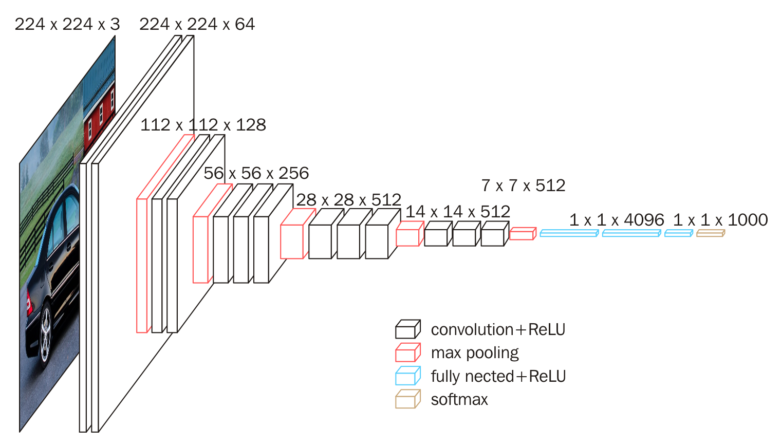
# 2.1 VGG 模型结构
下图是 VGG16 的具体结构示意图:
下面给出按照块划分的 VGG16 的结构图,可以结合上图进行理解:

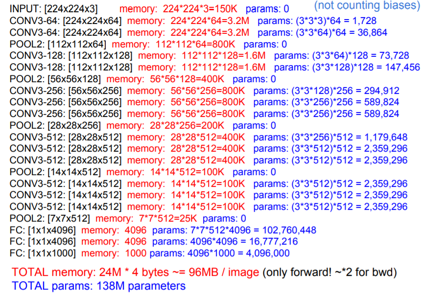
# 2.2 参数计算
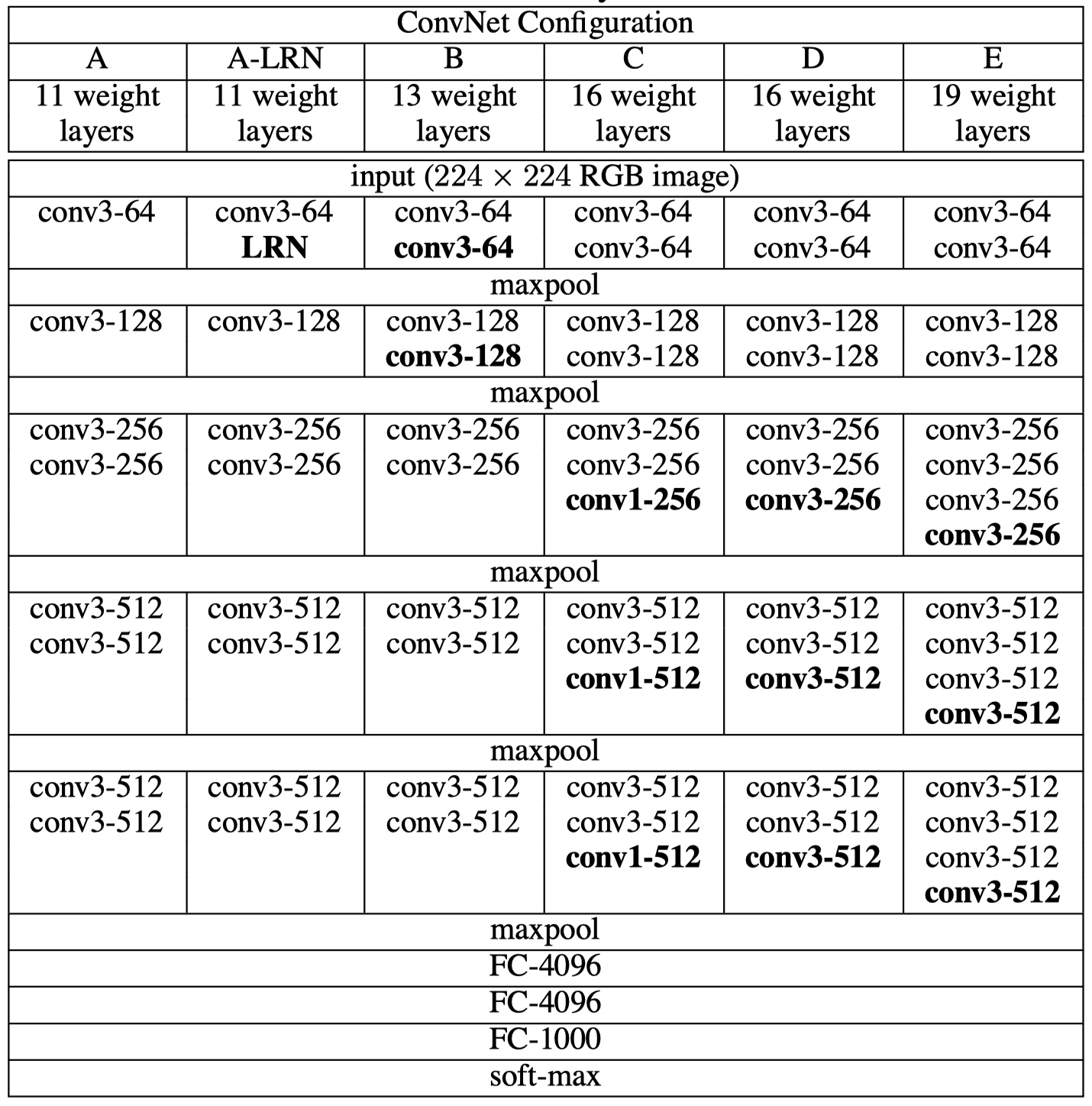
# 2.3 模型演变
共性
- 5 个 maxpool;
- maxpool 后,特征图通道数翻倍直至 512;
- 3 个 FC 层进行分类输出;
- maxpool 之间采用多个卷积层堆叠,对特征进行提取和抽象。
为什么从 11 层开始?
Goodfellow et al. (2014) applied deep ConvNets (11 weight layers) to the task of street number recognition.
演变过程
- A:11 层卷积
- A-LRN:基于 A 增加一个 LRN
- B:第 1、2 个 block 中增加 1 个 3 x 3 卷积
- C:第 3、4、5 个 block 分别增加 1 个 1 x 1 卷积,表明增加非线性有益于指标提升
- D:第 3、4、5 个 block 的 1 x 1 卷积替换为 3 x 3 卷积
- E:第 3、4、5 个 block 再分别增加 1 个 3 x 3 卷积
# 三、VGG 特点
# 3.1 堆叠 3 x 3 卷积核
- 增大感受野
- 2 个 3 x 3 堆叠等价于 1 个 5 x 5;
- 3 个 3 x 3 堆叠等价于 1 个 7 x 7;
- 增加非线性激活函数,增加特征抽象能力;
- 减少训练参数;
- 可看成 7 x 7 卷积核的正则化,强迫 7 x 7 分解为 3 x 3。
假设输入,输出通道均为 C 个通道,则
- 一个 7 x 7 卷积核所需参数量:
- 三个 3 x 3 卷积核所需参数量:
参数减少比例为:
# 3.2 尝试 1 x 1 卷积
借鉴 NIN,引入了 1 x 1 卷积,增加非线性激活函数,提升模型效果。
# 四、训练技巧
# 4.1 Scale jittering(尺寸扰动)
- 按比例缩放图片至最小边 S;
- 随机位置裁剪出 224 x 224 区域;
- 随机进行水平翻转。
S 设置方法:
- 固定值:固定为 256 或 384;
- 随机值:每个 batch 的 S 在 [256, 512],实现尺寸扰动。
# 4.2 预训练模型
深度神经网络对初始化敏感,可以用已训练好的模型参数进行初始化,可以避免梯度消失、梯度爆炸等训练难的问题。
- 深度加深时,用浅层网络初始化,即 B、C、D、E 用 A 模型初始化。
- Multi-scale 训练时,用小尺度初始化:
- 当 S = 384 时,用 S = 256 模型初始化;
- 当 S = [256, 512] 时,用 S = 384 模型初始化。
# 五、测试技巧
# 5.1 多尺度测试
- 图片等比例缩放至最短边 Q;
- 设置 3 个 Q,对图片进行预测,取平均。
Q 设置方法:
- 当 S 为固定值时,Q = (S - 32, S, S + 32);
- 当 S 为随机值时,Q = (S_min, 0.5 * (S_min + S_max), S_max)。
# 5.2 Dense test(稠密测试)
Dense test(稠密测试):将 FC 层转换为卷积操作,变为全卷积网络,实现任意尺寸图片输入。
- 经过全卷积网络得到 N x N x 1000 特征图;
- 在通道维度上求和(sum pooling)计算平均值,得到 1 x 1000 的输出向量。
# 5.3 Multi-Crop 测试
借鉴 AlexNet 与 GoogLeNet,对图片进行 Multi-Crop,裁剪大小为 224 x 224,并水平翻转。
1 张图,缩放至三种尺寸,然后每种尺寸裁剪出 50 张图片,之后再水平翻转,得到的图片总数为:
# 六、实验结果及分析
# 6.1 Single scale evaluation
方法
- 当 S 为固定值时:Q = S
- 当 S 为随机值时:Q = 0.5 * (S_min + S_max)
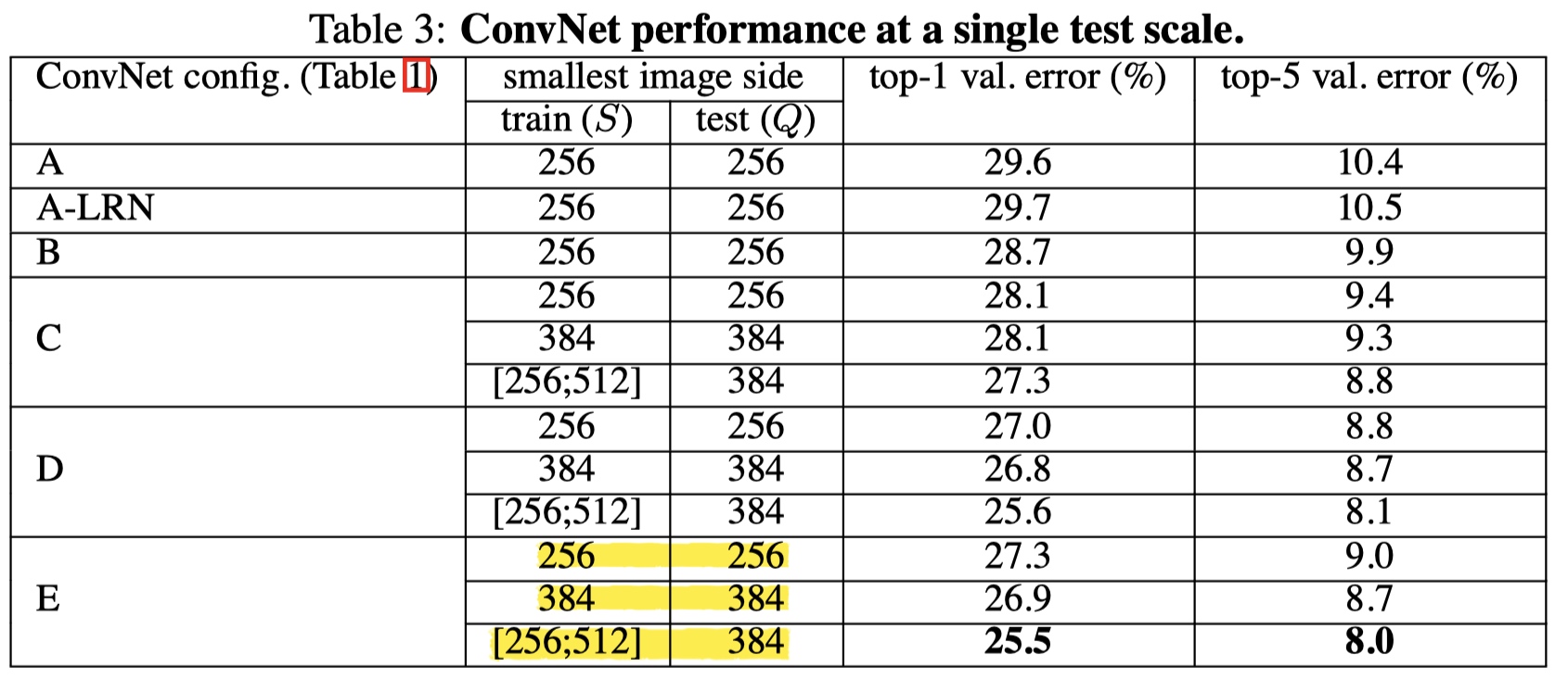
结论
- 误差随深度加深而降低,当模型到达 19 层时,误差饱和,不再下降;
- 增加 1 x 1 有助于性能提升(C(1) 与 A、B 对比);
- 训练时加入尺度扰动,有助于性能提升(C、D、E 的 (3) 与 (1)、(2) 对比);
- 论文中还提到,将 2 个 3 x 3 替换为1 个 5 x 5,top1 精度下降 7%,说明堆叠使用 3 x 3 有助于性能提升。
# 6.2 Multi scale evaluation
方法
- 当 S 为固定值时,Q = (S - 32, S, S + 32);
- 当 S 为随机值时,Q = (S_min, 0.5 * (S_min + S_max), S_max)。
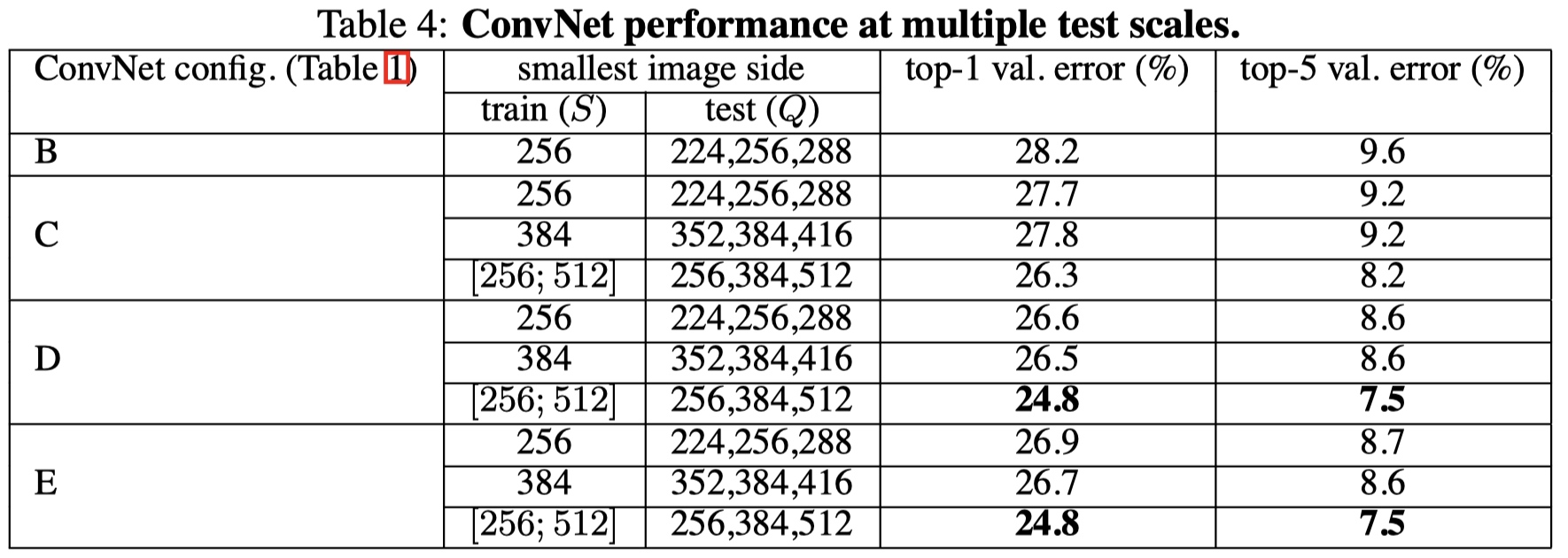
结论
- 多尺度测试有助于性能提升。
# 6.3 Multi crop evaluation
方法
等步长的滑动 224 x 224 的窗口进行裁剪,在尺度为 Q 的图像上裁剪 5 * 5 = 25 张图片,然后再进行水平翻转,得到 50 张图片,结合三个 Q 值,一张图片得到 150 张图片输入到模型中。
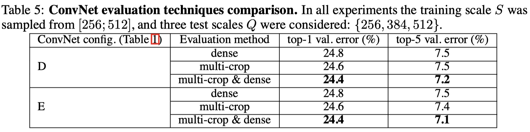
结论
- Multi-Crop 优于 Dense;
- Multi-Crop 结合 Dense,可形成互补(边界信息的互补),达到最优结果。
# 6.4 Convnet fusion
方法
ILSVRC 中,多模型融合已经是常规操作,ILSVRC 中提交的模型为 7 个模型融合。
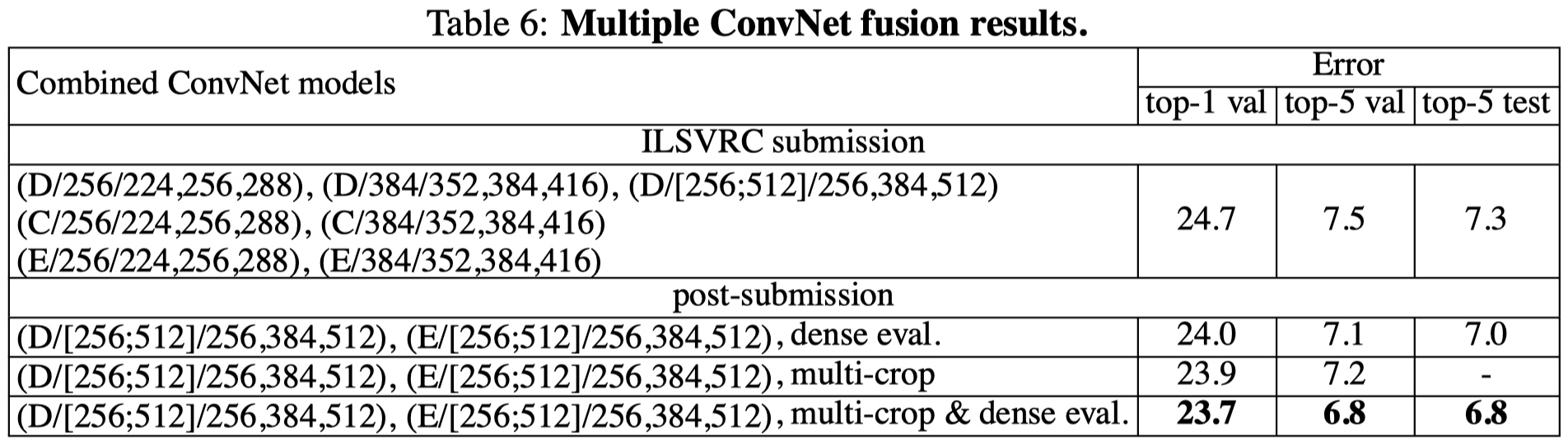
结论
采用最优的两个模型
- D/[256, 512]/256,384,512
- E/[256, 512]/256,384,512
结合 Multi-Crop 和 Dense,可得到最优结果。
# 6.5 Comparison with the state of the art

结论
- 单模型时,VGG 优于冠军 GoogLeNet。
# 七、论文总结
# 7.1 关键点 & 创新点
- 堆叠小卷积核,加深网络;
- 训练阶段,尺度扰动;
- 测试阶段,多尺度及 Multi-Crop + Dense。
# 7.2 启发点
采用小卷积核,获得高精度。
achieve better accuracy. For instance, the best-performing submissions to the ILSVRC- 2013 (Zeiler & Fergus, 2013; Sermanet et al., 2014) utilised smaller receptive window size and smaller stride of the first convolutional layer. (1 Introduction p2)
采用多尺度及稠密预测,获得高精度。
Another line of improvements dealt with training and testing the networks densely over the whole image and over multiple scales. (1 Introduction p2)
1 x 1 卷积可认为是线性变换,同时增加非线性层。
In one of the configurations we also utilise 1 × 1 convolution filters, which can be seen as a linear transformation of the input channels (followed by non-linearity). (2.1 Architecture p1)
填充大小准则:保持卷积后特征图分辨率不变。
the spatial padding of conv. layer input is such that the spatial resolution is preserved after convolution (2.1 Architecture p1)
LRN 对精度无提升。
such normalisation does not improve the performance on the ILSVRC dataset, but leads to increased memory con- sumption and computation time. (2.1 Architecture p3)
Xavier 初始化可达较好效果。
It is worth noting that after the paper submission we found that it is possible to initialise the weights without pre-training by using the random initialisation procedure of Glorot & Bengio (2010). (3.1 Trainning p2)
S 远大于 224,图片可能仅包含物体的一部分。
S ≫ 224 the crop will correspond to a small part of the image, containing a small object or an object part (3.1 Trainning p4)
大尺度模型采用小尺度模型初始化,可加快收敛。
To speed-up training of the S = 384 network, it was initialised with the weights pre-trained with S = 256, and we used a smaller initial learning rate of 0.001. (3.1 Trainning p5)
物体尺寸不一,因此采用多尺度训练,可以提高精度。
Since objects in images can be of different size, multi scale training is beneficial to take this into account during training.(3.1 Trainning p6)
Multi-Crop 存在重复计算,因而低效。
there is no need to sample multiple crops at test time (Krizhevsky et al., 2012), which is less efficient as it requires network re-computation for each crop.(3.2 Testing p2)
Multi-Crop 可看成 Dense 的补充,因为它们边界处理有所不同。
Also, multi-crop evaluation is complementary to dense evaluation due to different convolution boundary conditions (3.2 Testing p2)
小而深的卷积网络优于大而浅的卷积网络。
which confirms that a deep net with small filters outperforms a shallow net with larger filters. (4.1 Single scale evaluation p3)
尺度扰动对训练和测试阶段有帮助。
The results, presented in Table 4, indicate that scale jittering at test time leads to better performance(4.2 Multi scale evaluation p2)